Estimate any function with Gradient Descent

We already described in Gradient Descent from scratch how we can find all 3 parameters of a single dimension quadratic function (ball height h for time t). Let’s now extend on that knowledge to see if we can optimise parameters with no prior knowledge of the underlying function of our data.

The function we used in our prior post was \(h(t)=−4.9t^2+20​t+30​\). Let’s try to approximate it in a generic way!

First attempt

We want to find the relationship between two one-dimension variables (x and y). It’s simplest form would be a constant relationship, i.e. for all values of x, f(x) does not change: \(f(x) = K\) where K can by any constant value. Most input data we want to predict isn’t constant values so that won’t work (our quadratic might hit the same y twice at most due to its simmetry but not more than that).

       +----------+
------>| constant |------>
   x   +----------+   K

As a second guess we can try a linear relationship where y changes linearly with x, i.e. \(f(x) = x\). Such a line has a slope of 1 and passes through the origin (y=0 when x=0) (more on lines here) so let’s parameterise it so we can move it around and be a bit more flexible:

\(f(x) = m*x + b\) where m is our slope and b is the Y-intercept

       +--------+
------>| linear |------>
   x   +--------+   y

Note: if the slope is 0 (m=0) it would be equivalent to having a constant as in our first idea, i.e. a parallel line to the x axis

This time we’ll rely on PyTorch to calculate the gradients so we don’t need to manually take derivatives for our loss function like we did in the previous post.

Let’s generate some data for the function we want to find (no noise in our y values this time for the sake of simplicity):

def generate_f(m, b, x): return m*x + b;
def f(x): return -4.9*(x**2) + 20*x + 30;

x = torch.arange(0, 10, 1);
y = f(x);

And execute GD for a simple line:

def line(m, b, x): return m*x + b;
def generate_line(m, b): return partial(line, m, b);

learning_rate = 0.01;
steps = 100;

params = tensor([1, 1]).float();
params.requires_grad_();

for i in range(steps):
    predicted_f = generate_line(*params)
    predicted_y = predicted_f(x)
    loss = F.l1_loss(y, predicted_y)
    loss.backward()
    with torch.no_grad(): params -= params.grad * learning_rate
    params.grad.zero_()

If we look at the behaviour of the loss in each iteration, we’ll see that we aren’t getting close enough to 0 (MAE = 30.6):

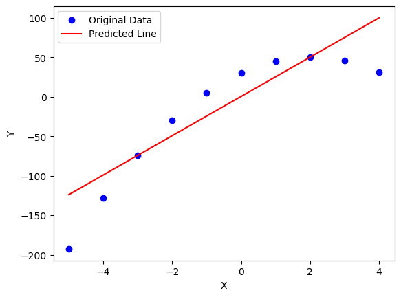
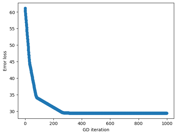
We could tweak our learning rate or steps number but will hardly lower much more the error rate since there is only so much we can do with a plain line.

Second attempt

Let’s see what happens if we apply a simple non-linear function on the output of the linear function we just tried. One such function is the ReLu which converts negative outputs to 0:

So we end up with a composite function like this:

       +--------+        +------+
------>| linear |------->| ReLu |------>
   x   +--------+   y'   +------+   y

Let’s run GD for this function, where only the optimised function changes:

-predicted_y = predicted_f(x)
+predicted_y = F.relu(predicted_f(x))

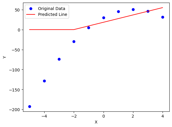
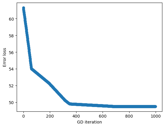
We actually worsened the loss adding the non-linear component in our example (MAE = 49.5) but something very powerful happened. The ReLu allowed GD to come up with a more complex shape that represents our input data:

Further refinements

As we can see just by adding a non-linear function we use we can allow Gradient Descent to come up with more flexible functions. Since the ReLu crops values below 0, we could add a horizontal line with no slope (m=0) to allow Gradient Descent to find values that would move our predictions in the negatives of the Y-axis:

       +--------+        +------+       +--------------+
------>| linear |------->| ReLu |------>| linear (m=0) |------>
   x   +--------+   y''  +------+   y'  +--------------+   y

The only change in our code would be to add an additional parameter from the new line \(f(x) = 0*x + b\):

-predicted_f = generate_line(*params)
-predicted_y = predicted_f(x)
+predicted_line_1 = generate_line(params[0], params[1])
+predicted_line_2 = generate_line(0, params[2])
+predicted_y = F.relu(predicted_line_1(x)) + predicted_line_2

Which would result in the following prediction:

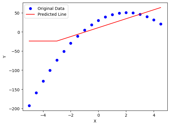
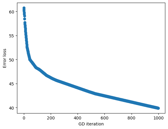
Notice how GD was able to figure out that it needed a negative Y-intercept for the last line we introduced so that our predictions would go down in the Y-axis.

With ths foundation we are able to increase the number of rectified linear units enough so that we can draw any function that resembles our input data (e.g. think of a voice waveform). It would be a matter of performing more computations on our errror minimisation function (while calculating the gradients of each parameter in each step) among other tricks.

The exact same process applies if we increased the number of independent variables (or input dimensions) for the function we are trying to find. It just becomes harder to visualise since we are going beyond the 2-D we are used to seeing in a coordinate plane (our output Y versus our input X).

This is a sample 3-D plot where a ReLu is applied on a 2 dimensional input (x and y). The main difference with a single dimension is that now Gradient Descent will be looking on more axes to find its way through the planes (if functions are linear). Check Khans’ Academy introduction to 3D graphs if you need help with multivariable visualisation.

We can abstract the Line + ReLu we implemented above and add some Neural Networks terms:

• Weight: the slope m of our linear function
• Bias: the y-intercept b of our linear function
• Activation function: in our case, we chose a ReLu
• Node: applies an activation function on the weighted sum of its inputs
• Connection: the lines connecting the nodes which apply a linear function

.-------. x weight1 + bias1   .------. x weight3 + bias3  .--------.
| input |-------------------->| node |------------------->| output |
.-------.                   | .------.                    .--------.
                            |
.-------. x weight2 + bias2 |
| input |-------------------+
.-------.

Since our node sums all weighted inputs, we could represent all biases sums with an additional input with a weight of 1. In our sample we have a final linear function (and bias) to adjust for our negative output values which would remain the same:

.-------. x weight1           .------. x 0 + bias1        .--------.
| input |-------------------->| node |------------------->| output |
.-------.                   | .------.                    .--------.
                            |
.-------. x weight2         |
| input |-------------------+
.-------.                   | 
                            |
.------.  x 1               |
| bias |--------------------+
.------.

Now we have seen some building blocks and how they work in our first Neural Network sample which equips us to resolve way more complex problems in a more generic fashion!